Why Sparse Structure Helps a Transformer Learn Its Second Skill

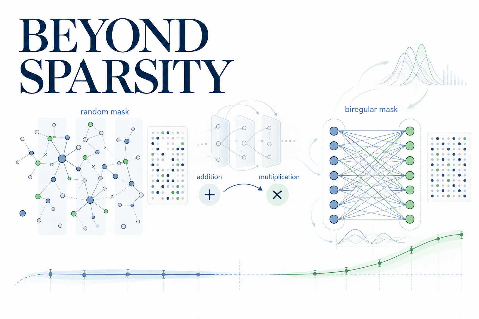
A transformer can learn modular addition perfectly and still struggle when multiplication is introduced next. In the experiments studied here, multiplication accuracy repeatedly stalls near 43%, even though the same architecture can sometimes learn the task. The obstacle is therefore not a simple lack of capacity.

The surprising intervention is made before training begins. Instead of changing the curriculum, optimizer, or loss, the researchers change which weights are allowed to exist. Random sparse masks help the model learn addition sooner, but masks built from biregular graphs do something more: at 97.7% sparsity, they raise the probability of fully learning multiplication from 4 out of 15 runs to 11 out of 15.

The result does not show that Ramanujan graphs generally make transformers more compositional. It comes from a 422,000-parameter model trained on arithmetic modulo 97. But it isolates a useful possibility: in sequential learning, connectivity may matter not only through how much capacity remains, but through how evenly that capacity is distributed.

The second task reaches a ceiling

Curriculum learning presents tasks in a deliberate order. In a sequential curriculum, the model first masters one task and only then encounters another. This resembles many practical settings: a pretrained model is adapted to a new domain, an agent acquires another tool, or a deployed system is updated without being rebuilt from scratch.

Sequential learning creates a tension. The parameters that encode the first skill become the starting point for the second. They may provide reusable structure, but they may also constrain optimization. A model can preserve the first task while failing to reorganize itself enough to learn the next one.

Castellon and Biswas study this tension in a deliberately controlled setting. Their model is a two-layer causal transformer with four attention heads, a model dimension of 128, and about 422,000 parameters. Each input has the form (a, operator, b, =), where the operator is addition or multiplication and the target is the result modulo 97.

There are 9,409 possible operand pairs for each operation. The model sees 40% of them during training and is evaluated on the remaining 60%. This unusual split is intentional: with limited training data and weight decay, small transformers often exhibit grokking. They first memorize the training examples; much later, validation accuracy abruptly rises as the model discovers a rule that generalizes.

The curriculum has two phases. In phase 1, the transformer trains only on addition until it groks. In phase 2, addition and multiplication batches are interleaved equally for 100,000 steps. A run is said to escape if multiplication validation accuracy reaches at least 95%.

Under dense initialization, most runs do not escape. The median multiplication accuracy stops at 43%, and only 4 of 30 runs cross the 95% threshold. The authors call this persistent plateau the sequential curriculum ceiling.

Sparsity is not one intervention

A sparse layer removes most of the possible connections between its inputs and outputs. If a weight matrix is represented by $W$ and a binary mask by $M$, the effective matrix is:

$$W_{\mathrm{eff}} = M \odot W$$

Here, $M_{ij}=1$ means that the connection from input coordinate $j$ to output coordinate $i$ remains active, $M_{ij}=0$ removes it, and $\odot$ denotes element-wise multiplication.

Two masks can have the same fraction of zeros and still define very different computational structures. The experiments compare two constructions at sparsities of 90%, 95%, and 97.7%.

Unstructured masks

In the unstructured condition, every weight is kept independently with probability $1-s$, where $s$ is the sparsity. This is a Bernoulli mask. It matches the total expected number of active weights, but it does not control how those weights are distributed. Some rows or columns may receive many connections, while others receive few or none.

Biregular Ramanujan masks

The structured condition treats a weight matrix as the adjacency matrix of a bipartite graph. Inputs form one set of vertices and outputs form the other. The graph is biregular: every input has the same number of outgoing connections, and every output has the same number of incoming connections.

The selected graphs also satisfy a Ramanujan spectral bound. In broad terms, this certifies near-optimal expansion: even with few edges, the graph mixes information efficiently. For a $(c,d)$-biregular graph, the paper studies the margin

$$\Delta_R = \sqrt{c-1} + \sqrt{d-1} - \lambda_2,$$

where $c$ and $d$ are the fixed degrees on the two sides and $\lambda_2$ is the second-largest singular value of the bipartite adjacency matrix. A non-negative margin indicates that the construction meets the relevant Ramanujan criterion.

These masks are applied to the query, key, value, and output projections in attention, and to the feed-forward down-projection. The token embeddings and feed-forward up-projection remain dense. Training otherwise stays unchanged.

Sparsity speeds grokking, but structure changes escape

The first result separates an effect of sparsity from an effect of topology. Every sparse condition learns addition faster than the dense model. The dense median grokking step is about 3,500; sparse medians range from 1,000 to 2,050 steps. At matched sparsity, however, there is no statistically significant difference between biregular and unstructured masks.

This is an observed result: sparsity shortens the memorization phase. It does not support the stronger interpretation that Ramanujan structure is responsible for the faster grokking.

The second phase produces a different pattern.

Initialization	Runs	Escapes at >=95%	Mean ceiling	Median ceiling
Dense	30	4/30	0.45	0.43
Biregular, 90% sparse	15	8/15	0.76	0.95
Biregular, 95% sparse	15	8/15	0.83	1.00
Biregular, 97.7% sparse	15	11/15	0.92	1.00
Unstructured, 90% sparse	15	4/15	0.62	0.45
Unstructured, 95% sparse	15	5/15	0.72	0.67
Unstructured, 97.7% sparse	15	4/15	0.79	0.87

Multiplication validation accuracy after the phase transition. Each structured and unstructured condition uses the same matched subset of 15 seeds; the dense baseline uses 30 runs.

For biregular masks, the escape rate rises from 8/15 at 90% sparsity to 11/15 at 97.7%. For unstructured masks, it remains essentially flat: 4/15, 5/15, and 4/15. At 97.7% sparsity, the difference between the two mask types is significant under the preregistered primary comparison: a one-sided Fisher exact test gives $p=0.013$, and a paired Wilcoxon signed-rank test on the ceiling values gives $p=0.008$.

The lower-sparsity comparisons point in the same direction but use only 15 runs per condition and are individually underpowered. They should not be read as independently established effects.

The careful conclusion is therefore narrower than “sparse models transfer better.” Matched unstructured sparsity does not reproduce the escape-rate improvement. At the most extreme sparsity tested, the pattern of the surviving connections matters.

Why random masks break down at high sparsity

At 97.7% sparsity, an unstructured 128-by-128 mask can leave complete rows or columns empty. The expected number of zero rows is approximately

$$128 \times 0.977^{128} \approx 6.5.$$

The factor $0.977^{128}$ is the probability that all 128 entries in a given row are removed. Multiplying by 128 gives the expected count across the matrix. In the actual networks, the unstructured 97.7%-sparse condition contains an average of 49 isolated row or column incidences across the masked attention projections of one transformer block.

Biregularity prevents this by construction. Every coordinate receives a fixed nonzero degree, so there are neither isolated units nor unusually connected hubs.

This difference also appears in the shape of the outcomes. At 97.7% sparsity, 67% of unstructured runs finish in a partial-escape range between 50% and 95% accuracy. Only 27% of biregular runs fall there; most either fail clearly or reach full generalization.

That bimodality is an exploratory, post-hoc observation, not a preregistered result. Still, it motivates a concrete hypothesis. Uneven random connectivity may preserve enough signal for the model to learn part of the multiplication rule while blocking the coordinated reorganization needed for complete generalization. A biregular mask removes that particular bottleneck.

The spectral explanation does not fit the data

Because the structured masks come from Ramanujan graphs, efficient spectral expansion is an obvious candidate mechanism. The data argue against that explanation.

As sparsity rises, the measured Ramanujan margin falls from 1.73 at 90% sparsity to 0.45 at 95% and just 0.03 at 97.7%. The largest escape advantage therefore occurs exactly where the margin is almost zero. Within each condition, the correlation between the second singular value and escape is also weak.

This does not prove that spectral properties are irrelevant in every setting. It shows that variation in this particular spectral margin does not explain the observed advantage. The paper’s leading alternative is degree uniformity: an even distribution of active connections may expose units more uniformly to the two tasks’ gradients.

The distinction matters. “Ramanujan initialization” bundles at least two properties—spectral expansion and fixed degrees. The experiment identifies an effect of the bundled construction, then uses the spectral diagnostic to make expansion less plausible. It does not yet isolate degree uniformity causally.

Embeddings are necessary, but they are not the whole story

A shared embedding table is one possible source of the ceiling. Addition and multiplication use the same integer tokens, so learning the second operation may require moving representations that have already specialized for the first.

The authors test this with an ablation. Starting from the same addition-trained checkpoints, they either allow the embeddings to keep learning during phase 2 or freeze them.

With trainable embeddings, the structural difference becomes stronger: 13 of 15 biregular runs escape, compared with 4 of 15 unstructured runs and 1 of 15 dense runs. With frozen embeddings, none of the three conditions escapes.

This establishes a dependency, not a complete mechanism. Embedding updates are necessary for escape in this setup. Yet embeddings alone do not determine the outcome, because changing the sparse structure outside the embedding table changes the escape rate when the embeddings are free to co-adapt.

The open problem is to explain that interaction. One possibility is that fixed-degree connectivity distributes gradient influence more evenly through the attention and feed-forward pathways, allowing the embeddings to reorganize without a few hub units dominating the update. The current experiments do not directly measure or manipulate that process.

What this result means for larger systems

The paper provides evidence for a rate shift, not a new learning regime. Dense and unstructured models occasionally learn multiplication too. Biregular initialization makes a successful outcome more likely and reduces the number of ambiguous partial solutions.

For research, the main contribution is methodological. Comparisons between dense and sparse networks often conflate two changes: the number of trainable connections and their arrangement. Here, matched sparsity separates them. Reduced capacity explains faster addition grokking; connectivity structure explains the additional change in sequential escape.

For production systems, the work suggests a hypothesis worth testing. Sparse fine-tuning, continual learning, and modular model updates all depend on how new gradients travel through a network that already encodes prior behavior. If active connections are distributed unevenly, some coordinates may become bottlenecks or hubs. Degree-controlled sparsity could offer a static architectural constraint that reduces this imbalance without adding a new training objective.

Initialization can shape what remains learnable

The initial question was why a transformer that has mastered one arithmetic operation can remain stuck on a second. This study does not give a complete mechanistic answer, but it narrows the possibilities.

Sparsity alone makes the first task grok faster. Biregular connectivity changes the probability and shape of success on the second. The benefit disappears when embeddings cannot adapt, while the graph’s spectral margin does not track the effect. The strongest remaining explanation is that uniform degrees prevent disconnected or disproportionately influential units and thereby support embedding co-adaptation.

Whether this principle survives at larger scale is open. The broader lesson is already useful: an initialization mask is not merely a compression device. By deciding where gradients can flow, it can influence which skills a trained model is still able to acquire.

Sources

• Clément Castellon and Arindam Biswas, Biregular Sparse Initialization Shifts the Rate and Shape of Compositional Escape in Sequential Arithmetic Curricula, Workshop on Compositional Learning at ICML 2026.
• Alethea Power et al., Grokking: Generalization Beyond Overfitting on Small Algorithmic Datasets, 2022.
• Neel Nanda et al., Progress Measures for Grokking via Mechanistic Interpretability, 2023.
• Shlomo Hoory, Nathan Linial, and Avi Wigderson, Expander Graphs and Their Applications, Bulletin of the American Mathematical Society, 2006.